Tidy Tuesday Exercise 2

Let’s load the data and other packages. We’ll use the tidytuesdayR package to do this.

library(tidyverse)
Warning: package 'tidyverse' was built under R version 4.2.2
Warning: package 'ggplot2' was built under R version 4.2.2
Warning: package 'tibble' was built under R version 4.2.2
Warning: package 'tidyr' was built under R version 4.2.2
Warning: package 'readr' was built under R version 4.2.2
Warning: package 'purrr' was built under R version 4.2.2
Warning: package 'dplyr' was built under R version 4.2.2
Warning: package 'stringr' was built under R version 4.2.2
Warning: package 'forcats' was built under R version 4.2.2
Warning: package 'lubridate' was built under R version 4.2.2
── Attaching core tidyverse packages ──────────────────────── tidyverse 2.0.0 ──
✔ dplyr     1.1.0     ✔ readr     2.1.4
✔ forcats   1.0.0     ✔ stringr   1.5.0
✔ ggplot2   3.4.1     ✔ tibble    3.2.0
✔ lubridate 1.9.2     ✔ tidyr     1.3.0
✔ purrr     1.0.1     
── Conflicts ────────────────────────────────────────── tidyverse_conflicts() ──
✖ dplyr::filter() masks stats::filter()
✖ dplyr::lag()    masks stats::lag()
ℹ Use the conflicted package (<http://conflicted.r-lib.org/>) to force all conflicts to become errors
library(lubridate)
library(tidymodels)
Warning: package 'tidymodels' was built under R version 4.2.2
── Attaching packages ────────────────────────────────────── tidymodels 1.0.0 ──
✔ broom        1.0.4     ✔ rsample      1.1.1
✔ dials        1.1.0     ✔ tune         1.0.1
✔ infer        1.0.4     ✔ workflows    1.1.3
✔ modeldata    1.1.0     ✔ workflowsets 1.0.0
✔ parsnip      1.0.4     ✔ yardstick    1.1.0
✔ recipes      1.0.5     
Warning: package 'broom' was built under R version 4.2.2
Warning: package 'dials' was built under R version 4.2.2
Warning: package 'scales' was built under R version 4.2.2
Warning: package 'infer' was built under R version 4.2.2
Warning: package 'modeldata' was built under R version 4.2.2
Warning: package 'parsnip' was built under R version 4.2.2
Warning: package 'recipes' was built under R version 4.2.2
Warning: package 'rsample' was built under R version 4.2.2
Warning: package 'tune' was built under R version 4.2.2
Warning: package 'workflows' was built under R version 4.2.2
Warning: package 'workflowsets' was built under R version 4.2.2
Warning: package 'yardstick' was built under R version 4.2.2
── Conflicts ───────────────────────────────────────── tidymodels_conflicts() ──
✖ scales::discard() masks purrr::discard()
✖ dplyr::filter()   masks stats::filter()
✖ recipes::fixed()  masks stringr::fixed()
✖ dplyr::lag()      masks stats::lag()
✖ yardstick::spec() masks readr::spec()
✖ recipes::step()   masks stats::step()
• Use tidymodels_prefer() to resolve common conflicts.
library(tidytuesdayR)
Warning: package 'tidytuesdayR' was built under R version 4.2.2
tuesdata <- tidytuesdayR::tt_load('2023-04-11')
--- Compiling #TidyTuesday Information for 2023-04-11 ----
--- There are 2 files available ---
--- Starting Download ---

    Downloading file 1 of 2: `egg-production.csv`
    Downloading file 2 of 2: `cage-free-percentages.csv`
--- Download complete ---
eggproduction <- tuesdata$`egg-production`
cagefreepercentages <- tuesdata$`cage-free-percentages`

I’ve copied the following data dictionary from the TiduTuesday GitHub to reference more easily.

Data Dictionary

egg-production.csv

variable class description
observed_month double Month in which report observations are collected,Dates are recorded in ISO 8601 format YYYY-MM-DD
prod_type character type of egg product: hatching, table eggs
prod_process character type of production process and housing: cage-free (organic), cage-free (non-organic), all. The value ‘all’ includes cage-free and conventional housing.
n_hens double number of eggs produced by hens for a given month-type-process combo
n_eggs double number of hens producing eggs for a given month-type-process combo
source character Original USDA report from which data are sourced. Values correspond to titles of PDF reports. Date of report is included in title.

cage-free-percentages.csv

variable class description
observed_month double Month in which report observations are collected,Dates are recorded in ISO 8601 format YYYY-MM-DD
percent_hens double observed or computed percentage of cage-free hens relative to all table-egg-laying hens
percent_eggs double computed percentage of cage-free eggs relative to all table eggs,This variable is not available for data sourced from the Egg Markets Overview report
source character Original USDA report from which data are sourced. Values correspond to titles of PDF reports. Date of report is included in title.

Let’s start be taking a look at the data

glimpse(eggproduction)
Rows: 220
Columns: 6
$ observed_month <date> 2016-07-31, 2016-08-31, 2016-09-30, 2016-10-31, 2016-1…
$ prod_type      <chr> "hatching eggs", "hatching eggs", "hatching eggs", "hat…
$ prod_process   <chr> "all", "all", "all", "all", "all", "all", "all", "all",…
$ n_hens         <dbl> 57975000, 57595000, 57161000, 56857000, 57116000, 57750…
$ n_eggs         <dbl> 1147000000, 1142700000, 1093300000, 1126700000, 1096600…
$ source         <chr> "ChicEggs-09-23-2016.pdf", "ChicEggs-10-21-2016.pdf", "…
glimpse(cagefreepercentages)
Rows: 96
Columns: 4
$ observed_month <date> 2007-12-31, 2008-12-31, 2009-12-31, 2010-12-31, 2011-1…
$ percent_hens   <dbl> 3.20000, 3.50000, 3.60000, 4.40000, 5.40000, 6.00000, 5…
$ percent_eggs   <dbl> NA, NA, NA, NA, NA, NA, NA, NA, NA, NA, 9.634938, NA, 9…
$ source         <chr> "Egg-Markets-Overview-2019-10-19.pdf", "Egg-Markets-Ove…

It seems like these datasets span a different range of years. Let’s verify this.

eggproduction %>% 
  arrange(observed_month) %>%
  slice(c(1, n())) %>%
  bind_rows()
# A tibble: 2 × 6
  observed_month prod_type     prod_process          n_hens     n_eggs source   
  <date>         <chr>         <chr>                  <dbl>      <dbl> <chr>    
1 2016-07-31     hatching eggs all                 57975000 1147000000 ChicEggs…
2 2021-02-28     table eggs    cage-free (organic) 17491500  386912160 PY202103…
cagefreepercentages %>% 
  arrange(observed_month) %>%
  slice(c(1, n())) %>%
  bind_rows()
# A tibble: 2 × 4
  observed_month percent_hens percent_eggs source                             
  <date>                <dbl>        <dbl> <chr>                              
1 2007-12-31              3.2           NA Egg-Markets-Overview-2019-10-19.pdf
2 2021-02-28             29.2           NA Egg-Markets-Overview-2021-03-05.pdf

The cage-free percentages data goes back to 2007, while the egg production data only goes back to 2016. The most recent observations in both datasets is Feb. 28, 2021.

My data with the hypothesis that the number of eggs produced per hen differs based on the type of egg product (hatchling or table eggs).

H0: There is no difference between the number of eggs produced per hen. HA: There is a difference between the number of eggs produced per hen, and table eggs are produced at higher rates compared to hatchling eggs.

The outcome interest is the rate of egg production, which I will name rate_prod for rate of production.

eggproduction <- eggproduction %>% 
  group_by(prod_type) %>% 
  mutate(rate_prod  = n_eggs/n_hens)

Let’s prepare the datasets for a merge, which will hopefully this will make things easy to work with. I’ll start by making a variable that pulls just the month and year from ‘observed_month’ to make merge the datasets more seamless.

cagefreepercentages <- cagefreepercentages %>% 
  mutate(mon_yr = format_ISO8601(observed_month, precision = "ym"),
         mon = format(observed_month, "%m"),
        mon = as.factor(mon)) #only month

eggproduction <- eggproduction %>% 
  mutate(mon_yr = format_ISO8601(observed_month, precision = "ym"), 
         mon = format(observed_month, "%m"),
        mon = as.factor(mon))

I’ll do a bit more tidying up by using the computed estimates and by removing unnecessary variables

cagefreepercentages_clean <- cagefreepercentages %>% 
  filter(source == "computed")%>% 
  select(-c(observed_month, source))

eggproduction_clean <- eggproduction %>% 
  select(-c(observed_month, source))

Now, we’ll use inner join to merge by the mon_yr only that appear in both datasets

eggs_df <- inner_join(eggproduction_clean, cagefreepercentages_clean, by = join_by(mon_yr, mon))

eggs_df <- eggs_df %>% 
  mutate(prod_type = as.factor(prod_type),
         prod_process = as.factor(prod_process))

eggs_df$prod_type <- relevel(eggs_df$prod_type, ref = "table eggs")

#eggs_clean <- eggs_df %>% select(-mon_yr)

Let’s split the data into test and train

## setting the seed 
set.seed(123)
## Put 3/4 of the data into the training set 
data_split <- initial_split(eggs_df, prop = 3/4)

# Create data frames for the two sets:
train_data <- training(data_split)
test_data <- testing(data_split)

egg_metrics <- metric_set(accuracy, roc_auc, mn_log_loss)

#Cross validation
set.seed(123)
five_fold <- vfold_cv(train_data, v = 5, strata = prod_type)

Set the recipe

eggs_rec <- recipe(prod_type ~ prod_process + mon + rate_prod, data = train_data) %>% 
  step_dummy(prod_process, mon)

Now let’s set up a null model

null_mod <- null_model() %>% 
  set_engine("parsnip") %>% 
  set_mode("classification")

Null workflow

null_wflow <- workflow() %>%
  add_model(null_mod) %>%
  add_recipe(eggs_rec)
null_fit <- null_wflow %>% 
  fit(data = train_data)

null_fit %>%
  extract_fit_parsnip() %>%
  tidy()
# A tibble: 1 × 1
  value     
  <chr>     
1 table eggs

Decision Tree

library(rpart)

Attaching package: 'rpart'
The following object is masked from 'package:dials':

    prune
tune_spec <- 
  decision_tree(
    cost_complexity = tune(),
    tree_depth = tune()) %>% 
  set_engine("rpart") %>% 
  set_mode("classification")

tree_grid <- grid_regular(cost_complexity(),
                          tree_depth(),
                          levels = 5)
## workflow for decision tree
tree_wf <- workflow() %>%
  add_model(tune_spec) %>%
  add_recipe(eggs_rec)

tree_res <- 
  tree_wf %>% 
  tune_grid(resamples = five_fold,
    grid = tree_grid) 
tree_res %>% 
  collect_metrics() 
# A tibble: 50 × 8
   cost_complexity tree_depth .metric  .estimator  mean     n std_err .config   
             <dbl>      <int> <chr>    <chr>      <dbl> <int>   <dbl> <chr>     
 1    0.0000000001          1 accuracy binary         1     5       0 Preproces…
 2    0.0000000001          1 roc_auc  binary         1     5       0 Preproces…
 3    0.0000000178          1 accuracy binary         1     5       0 Preproces…
 4    0.0000000178          1 roc_auc  binary         1     5       0 Preproces…
 5    0.00000316            1 accuracy binary         1     5       0 Preproces…
 6    0.00000316            1 roc_auc  binary         1     5       0 Preproces…
 7    0.000562              1 accuracy binary         1     5       0 Preproces…
 8    0.000562              1 roc_auc  binary         1     5       0 Preproces…
 9    0.1                   1 accuracy binary         1     5       0 Preproces…
10    0.1                   1 roc_auc  binary         1     5       0 Preproces…
# … with 40 more rows
#visualize
tree_res %>%
  autoplot()

#Selecting the best tree using rmse.
best_tree <- tree_res %>%
  select_best(metric = "roc_auc") 

I am unsure if I am interpretting this correctly, but it seems like accuracy and ROC_AUC were perfect?

Logistic regression

log_spec <- logistic_reg() %>%
  set_engine(engine = "glm") %>%
  set_mode("classification")

Creating workflow object for logistic regression

log_wflow <- 
   workflow() %>% 
   add_recipe(eggs_rec) %>% 
   add_model(log_spec)

Creating trained workflow

logreg_fit <- log_wflow %>% 
  fit(data = train_data)
Warning: glm.fit: algorithm did not converge
Warning: glm.fit: fitted probabilities numerically 0 or 1 occurred

Pulling model fit

logreg_fit %>% 
  extract_fit_parsnip()  
parsnip model object


Call:  stats::glm(formula = ..y ~ ., family = stats::binomial, data = data)

Coefficients:
                         (Intercept)                             rate_prod  
                            237.5439                              -10.7688  
prod_process_cage.free..non.organic.      prod_process_cage.free..organic.  
                            -14.2449                              -14.2947  
                             mon_X02                               mon_X03  
                            -21.6212                               -0.8866  
                             mon_X04                               mon_X05  
                             -7.6954                                0.4962  
                             mon_X06                               mon_X07  
                             -7.1329                                0.3517  
                             mon_X08                               mon_X09  
                              1.8642                               -7.1652  
                             mon_X10                               mon_X11  
                              0.5256                               -5.8567  
                             mon_X12  
                              0.1296  

Degrees of Freedom: 161 Total (i.e. Null);  147 Residual
Null Deviance:      185.4 
Residual Deviance: 1.26e-09     AIC: 30

Random forest

library(ranger)
Warning: package 'ranger' was built under R version 4.2.3
rf_spec <- 
  rand_forest(min_n = tune()) %>% 
  set_engine("ranger", importance = "impurity") %>% 
  set_mode("classification")

Random forest workflow

rf_wflow <- workflow() %>%
 add_recipe(eggs_rec) %>% 
 add_model(rf_spec) 

Fit a model

rf_wflow_fit <- rf_wflow %>% 
  fit(data = train_data)
Warning: tune samples were requested but there were 162 rows in the data. 162
will be used.
doParallel::registerDoParallel()

set.seed(345)
tune_res <- tune_grid(
  rf_wflow,
  resamples = five_fold,
  grid = 20)

#Visualize..
tune_res %>% 
  autoplot()

best_rf <-   tune_res %>% 
  select_best(metric = "roc_auc")

rf_final_wf <- rf_wflow %>%
  finalize_workflow(best_rf)

rf_final_wf %>% 
  fit(data = train_data)
══ Workflow [trained] ══════════════════════════════════════════════════════════
Preprocessor: Recipe
Model: rand_forest()

── Preprocessor ────────────────────────────────────────────────────────────────
1 Recipe Step

• step_dummy()

── Model ───────────────────────────────────────────────────────────────────────
Ranger result

Call:
 ranger::ranger(x = maybe_data_frame(x), y = y, min.node.size = min_rows(~36L,      x), importance = ~"impurity", num.threads = 1, verbose = FALSE,      seed = sample.int(10^5, 1), probability = TRUE) 

Type:                             Probability estimation 
Number of trees:                  500 
Sample size:                      162 
Number of independent variables:  14 
Mtry:                             3 
Target node size:                 36 
Variable importance mode:         impurity 
Splitrule:                        gini 
OOB prediction error (Brier s.):  0.01356042 

Same results as above…

Multinomial regression via neural net

# Specify a multinomial regression via nnet
multireg_spec <- multinom_reg(penalty = 1) %>% 
  set_engine("nnet") %>% 
  set_mode("classification")

#trying to set workflow
multireg_wf <- workflow() %>% 
  add_model(multireg_spec) %>% 
  add_recipe(eggs_rec)

# Train a multinomial regression model ##
set.seed(2056)
multireg_fit <- multireg_spec %>% 
  fit(prod_type ~ prod_process + mon + rate_prod, data = train_data)
  
#print model
multireg_fit %>%
  tidy()
# A tibble: 15 × 6
   y.level term                                estimate std.e…¹ statis…² p.value
   <chr>   <chr>                                  <dbl>   <dbl>    <dbl>   <dbl>
 1 1       (Intercept)                          2.37     1.95    1.21     0.225 
 2 1       prod_processcage-free (non-organic) -1.54     0.659  -2.34     0.0192
 3 1       prod_processcage-free (organic)     -1.64     0.639  -2.57     0.0101
 4 1       mon02                               -0.00993  1.12   -0.00888  0.993 
 5 1       mon03                                0.106    1.01    0.105    0.916 
 6 1       mon04                                0.0334   0.998   0.0335   0.973 
 7 1       mon05                                0.0692   0.998   0.0693   0.945 
 8 1       mon06                                0.188    1.04    0.180    0.857 
 9 1       mon07                                0.315    1.08    0.291    0.771 
10 1       mon08                                0.340    0.933   0.365    0.715 
11 1       mon09                                0.300    0.932   0.322    0.748 
12 1       mon10                                0.0470   0.992   0.0474   0.962 
13 1       mon11                                0.195    0.962   0.203    0.839 
14 1       mon12                                0.234    0.964   0.242    0.809 
15 1       rate_prod                           -0.144    0.0841 -1.71     0.0879
# … with abbreviated variable names ¹​std.error, ²​statistic

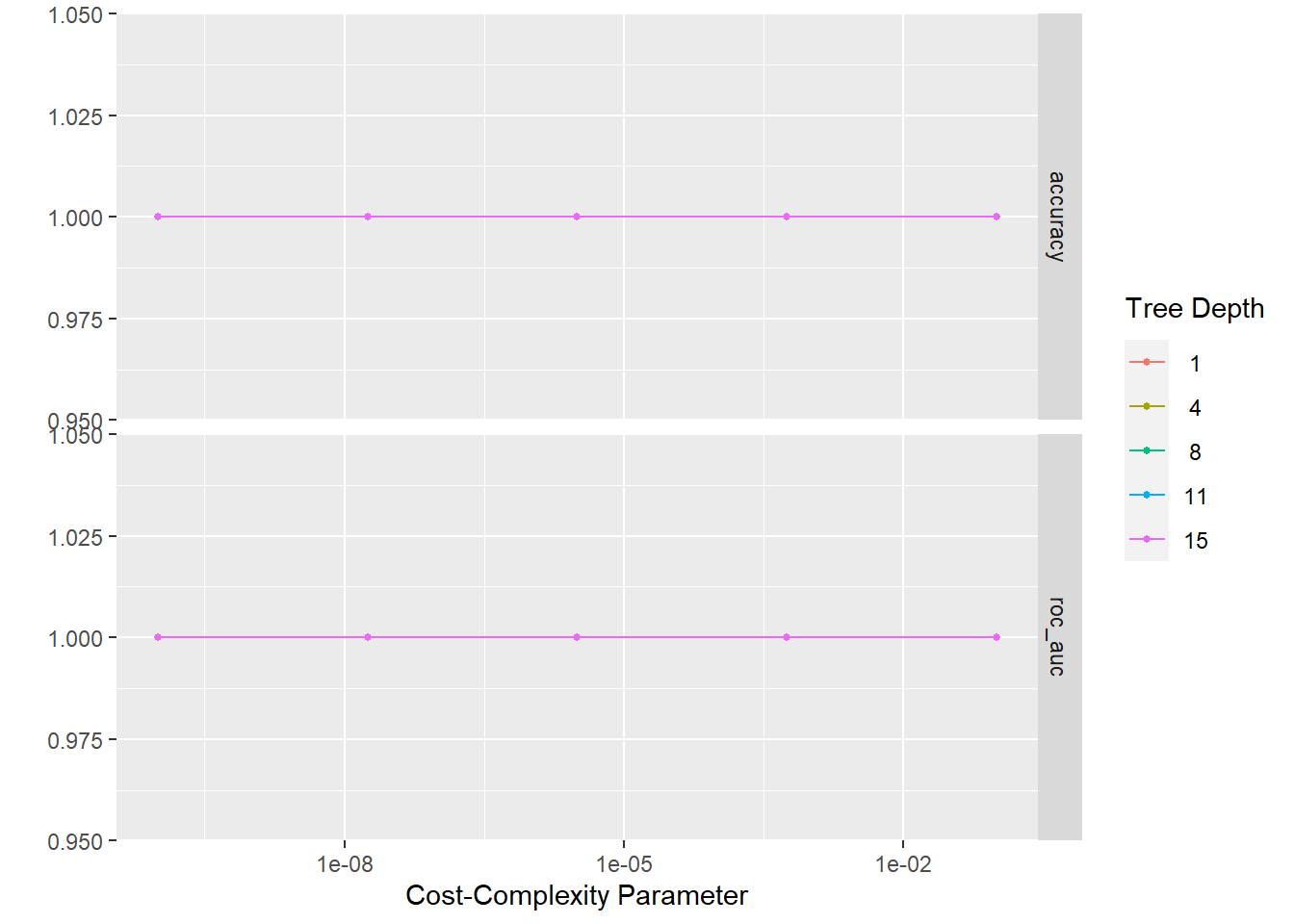
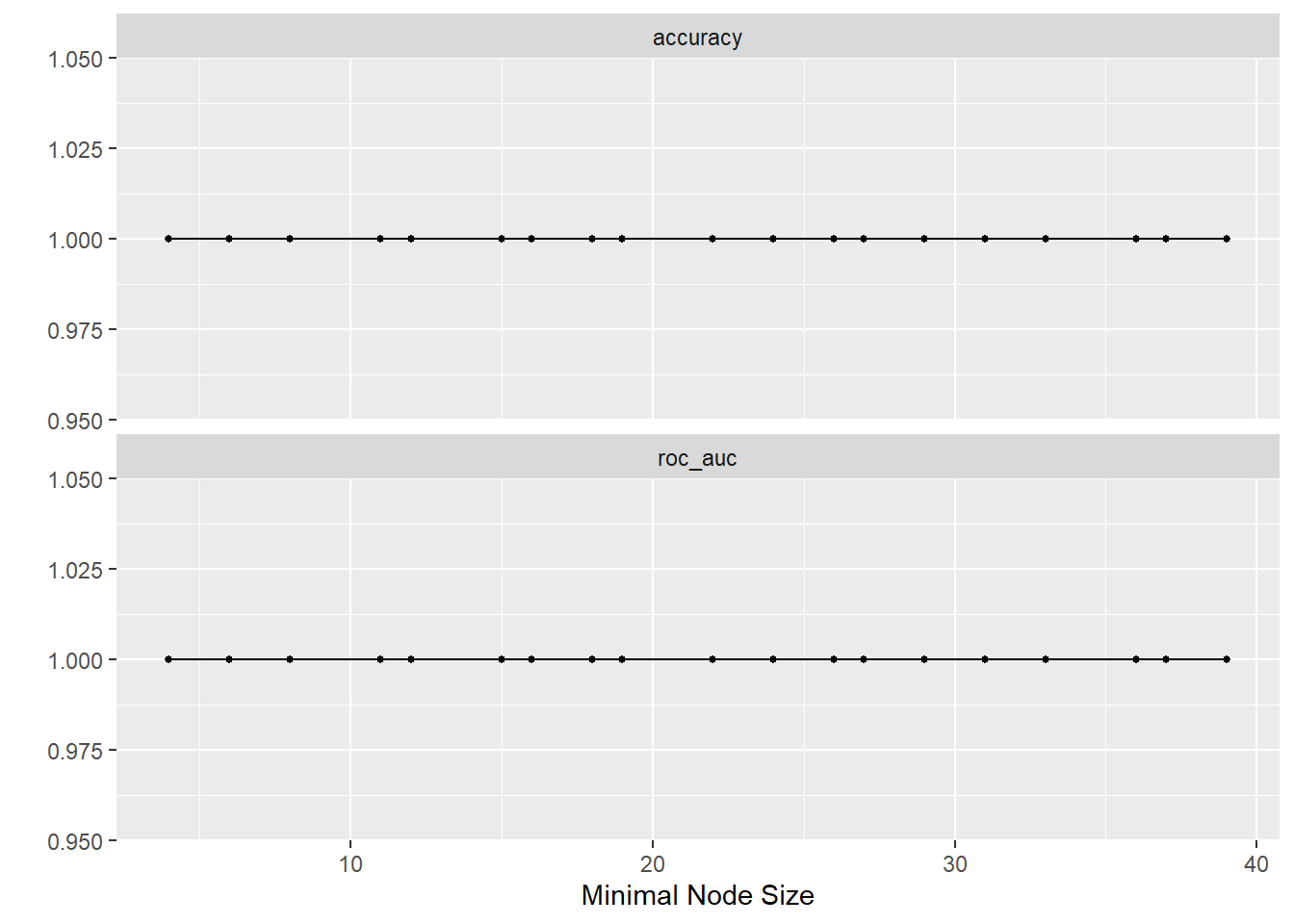
All the models appears to perform similarly… the logistic regression model is the might be the simplest model, so let’s use that to to test model performance against the test_data

# Make predictions for the test set
eggs_results <- test_data %>% 
  select(prod_type) %>% 
  bind_cols(logreg_fit %>% 
              predict(new_data = test_data)) %>% 
  bind_cols(logreg_fit %>% 
              predict(new_data = test_data, type = "prob"))

# Print predictions
eggs_results %>% 
  slice_head(n = 54)
# A tibble: 54 × 4
# Groups:   prod_type [2]
   prod_type  .pred_class `.pred_table eggs` `.pred_hatching eggs`
   <fct>      <fct>                    <dbl>                 <dbl>
 1 table eggs table eggs                1.00              1.62e-12
 2 table eggs table eggs                1.00              1.82e-11
 3 table eggs table eggs                1.00              3.74e-13
 4 table eggs table eggs                1                 2.22e-16
 5 table eggs table eggs                1.00              7.49e-10
 6 table eggs table eggs                1.00              2.27e-12
 7 table eggs table eggs                1                 2.22e-16
 8 table eggs table eggs                1                 2.22e-16
 9 table eggs table eggs                1.00              1.87e-12
10 table eggs table eggs                1                 2.22e-16
# … with 44 more rows
#Confusion matrix
conf_mat(eggs_results,
         truth = prod_type,
         estimate = .pred_class) 
# A tibble: 2 × 2
  prod_type     conf_mat  
  <fct>         <list>    
1 table eggs    <conf_mat>
2 hatching eggs <conf_mat>
## Did not work like expected...

#pulling accuracy
accuracy(eggs_results, 
         truth = prod_type,
         estimate = .pred_class)
# A tibble: 2 × 4
  prod_type     .metric  .estimator .estimate
  <fct>         <chr>    <chr>          <dbl>
1 table eggs    accuracy binary             1
2 hatching eggs accuracy binary             1
##Is 100% accurate

## trying to pull ROC-AUC to see if performance of predictive model is good
roc_auc(eggs_results,
        truth = prod_type,
        `.pred_hatching eggs`) 
Warning: There were 2 warnings in `dplyr::summarise()`.
The first warning was:
ℹ In argument: `.estimate = metric_fn(...)`.
ℹ In group 1: `prod_type = table eggs`.
Caused by warning:
! No control observations were detected in `truth` with control level 'hatching eggs'.
ℹ Run `dplyr::last_dplyr_warnings()` to see the 1 remaining warning.
# A tibble: 2 × 4
  prod_type     .metric .estimator .estimate
  <fct>         <chr>   <chr>          <dbl>
1 table eggs    roc_auc binary            NA
2 hatching eggs roc_auc binary            NA
##estimate is NA?

As far as I can tell, it seemed like the logistic regression model was able to predict prod_type perfectly. Intuitively, it seems like these models should not performed perfectly, but in looking at the data it is very clear that hens producing table eggs lay significantly more eggs than those producing hatching eggs. Unfortunately, my knowledge of tidymodels has limited my ability to troubleshoot potential issues in these classification models…